Overview
Today we will learn to:
Use the six main data frame manipulation ‘verbs’ with pipes in dplyr
Understand how group_by() and summarize() can be combined to summarize datasets
Analyze a subset of data using logical filtering
Questions
How can I manipulate data frames without repeating myself?
The Problem with Base R
We often need to select observations, group data, or calculate statistics.
Using base R:
<- read.csv ("https://raw.githubusercontent.com/swcarpentry/r-novice-gapminder/main/episodes/data/gapminder_data.csv" mean (gapminder$ gdpPercap[gapminder$ continent == "Africa" ])mean (gapminder$ gdpPercap[gapminder$ continent == "Americas" ])mean (gapminder$ gdpPercap[gapminder$ continent == "Asia" ])
This is repetitive and error-prone!
The dplyr Package
The dplyr package provides functions for manipulating data frames that:
Reduce repetition
Reduce probability of errors
Are easier to read
Tidyverse
dplyr belongs to the Tidyverse - a family of R packages designed for data science.
These packages work harmoniously together. Learn more at: tidyverse.org
The Five Main Verbs
We’ll cover these commonly used functions:
select() - choose columnsfilter() - choose rowsgroup_by() - group datasummarize() - calculate summariesmutate() - create new columns
Plus the pipe operator: %>%
Loading dplyr
If not installed, run: install.packages("dplyr")
Using select()
Keep only specific columns:
<- select (gapminder, year, country, gdpPercap)head (year_country_gdp)
  year     country gdpPercap
1 1952 Afghanistan  779.4453
2 1957 Afghanistan  820.8530
3 1962 Afghanistan  853.1007
4 1967 Afghanistan  836.1971
5 1972 Afghanistan  739.9811
6 1977 Afghanistan  786.1134
Removing Columns with select()
Use - to remove columns:
<- select (gapminder, - continent)head (smaller_gapminder)
      country year      pop lifeExp gdpPercap
1 Afghanistan 1952  8425333  28.801  779.4453
2 Afghanistan 1957  9240934  30.332  820.8530
3 Afghanistan 1962 10267083  31.997  853.1007
4 Afghanistan 1967 11537966  34.020  836.1971
5 Afghanistan 1972 13079460  36.088  739.9811
6 Afghanistan 1977 14880372  38.438  786.1134
Introduction to Pipes
The pipe symbol %>% passes data from one function to the next:
<- gapminder %>% select (year, country, gdpPercap)head (year_country_gdp)
  year     country gdpPercap
1 1952 Afghanistan  779.4453
2 1957 Afghanistan  820.8530
3 1962 Afghanistan  853.1007
4 1967 Afghanistan  836.1971
5 1972 Afghanistan  739.9811
6 1977 Afghanistan  786.1134
Understanding Pipes
Step by step:
Start with gapminder data frame
Pass it using %>% to the next step
select() receives the data automatically
Fun Fact: Similar to the shell pipe | but the concept is the same!
Renaming Columns
Use rename() within a pipeline:
<- year_country_gdp %>% rename (gdp_per_capita = gdpPercap)head (tidy_gdp)
  year     country gdp_per_capita
1 1952 Afghanistan       779.4453
2 1957 Afghanistan       820.8530
3 1962 Afghanistan       853.1007
4 1967 Afghanistan       836.1971
5 1972 Afghanistan       739.9811
6 1977 Afghanistan       786.1134
Syntax: rename(new_name = old_name)
Using filter()
Keep only rows that meet criteria:
<- gapminder %>% filter (continent == "Europe" ) %>% select (year, country, gdpPercap)head (year_country_gdp_euro)
  year country gdpPercap
1 1952 Albania  1601.056
2 1957 Albania  1942.284
3 1962 Albania  2312.889
4 1967 Albania  2760.197
5 1972 Albania  3313.422
6 1977 Albania  3533.004
Combining filter() Conditions
Filter with multiple conditions:
<- gapminder %>% filter (continent == "Europe" , year == 2007 ) %>% select (country, lifeExp)head (europe_lifeExp_2007)
                 country lifeExp
1                Albania  76.423
2                Austria  79.829
3                Belgium  79.441
4 Bosnia and Herzegovina  74.852
5               Bulgaria  73.005
6                Croatia  75.748
Challenge 1
Write a single command (which can span multiple lines and includes pipes) that will produce a data frame that has the African values for lifeExp, country and year, but not for other Continents.
How many rows does your data frame have and why?
Challenge 1 Solution
<- gapminder %>% filter (continent == "Africa" ) %>% select (year, country, lifeExp)nrow (year_country_lifeExp_Africa)
624 rows (52 African countries × 12 years of data)
Order of Operations
The order of operations matters!
If we used select() first, filter() would not be able to find the variable continent since we would have removed it.
Always filter before selecting when you need to filter on a column you won’t keep!
Using group_by()
Instead of filtering one group at a time, use group_by() to work with all groups:
'data.frame':   1704 obs. of  6 variables:
 $ country  : chr  "Afghanistan" "Afghanistan" "Afghanistan" "Afghanistan" ...
 $ year     : int  1952 1957 1962 1967 1972 1977 1982 1987 1992 1997 ...
 $ pop      : num  8425333 9240934 10267083 11537966 13079460 ...
 $ continent: chr  "Asia" "Asia" "Asia" "Asia" ...
 $ lifeExp  : num  28.8 30.3 32 34 36.1 ...
 $ gdpPercap: num  779 821 853 836 740 ...
group_by() Structure
str (gapminder %>% group_by (continent))
gropd_df [1,704 × 6] (S3: grouped_df/tbl_df/tbl/data.frame)
 $ country  : chr [1:1704] "Afghanistan" "Afghanistan" "Afghanistan" "Afghanistan" ...
 $ year     : int [1:1704] 1952 1957 1962 1967 1972 1977 1982 1987 1992 1997 ...
 $ pop      : num [1:1704] 8425333 9240934 10267083 11537966 13079460 ...
 $ continent: chr [1:1704] "Asia" "Asia" "Asia" "Asia" ...
 $ lifeExp  : num [1:1704] 28.8 30.3 32 34 36.1 ...
 $ gdpPercap: num [1:1704] 779 821 853 836 740 ...
 - attr(*, "groups")= tibble [5 × 2] (S3: tbl_df/tbl/data.frame)
  ..$ continent: chr [1:5] "Africa" "Americas" "Asia" "Europe" ...
  ..$ .rows    : list<int> [1:5]
  .. ..$ : int [1:624] 25 26 27 28 29 30 31 32 33 34 ...
  .. ..$ : int [1:300] 49 50 51 52 53 54 55 56 57 58 ...
  .. ..$ : int [1:396] 1 2 3 4 5 6 7 8 9 10 ...
  .. ..$ : int [1:360] 13 14 15 16 17 18 19 20 21 22 ...
  .. ..$ : int [1:24] 61 62 63 64 65 66 67 68 69 70 ...
  .. ..@ ptype: int(0)
  ..- attr(*, ".drop")= logi TRUE
Notice the grouped_df class - it’s now organized by continent!
Using summarize()
Combine group_by() with summarize() to calculate statistics per group:
<- gapminder %>% group_by (continent) %>% summarize (mean_gdpPercap = mean (gdpPercap))
# A tibble: 5 × 2
  continent mean_gdpPercap
  <chr>              <dbl>
1 Africa             2194.
2 Americas           7136.
3 Asia               7902.
4 Europe            14469.
5 Oceania           18622.
Challenge 2
Calculate the average life expectancy per country.
Which has the longest average life expectancy and which has the shortest average life expectancy?
Challenge 2 Solution
<- gapminder %>% group_by (country) %>% summarize (mean_lifeExp = mean (lifeExp))%>% filter (mean_lifeExp == min (mean_lifeExp) | mean_lifeExp == max (mean_lifeExp))
# A tibble: 2 × 2
  country      mean_lifeExp
  <chr>               <dbl>
1 Iceland              76.5
2 Sierra Leone         36.8
Challenge 2 Solution (using arrange)
Another way using arrange():
# Shortest life expectancy %>% arrange (mean_lifeExp) %>% head (1 )
# A tibble: 1 × 2
  country      mean_lifeExp
  <chr>               <dbl>
1 Sierra Leone         36.8
# Longest life expectancy %>% arrange (desc (mean_lifeExp)) %>% head (1 )
# A tibble: 1 × 2
  country mean_lifeExp
  <chr>          <dbl>
1 Iceland         76.5
Grouping by Multiple Variables
Group by more than one variable:
<- gapminder %>% group_by (continent, year) %>% summarize (mean_gdpPercap = mean (gdpPercap))head (gdp_bycontinents_byyear)
# A tibble: 6 × 3
# Groups:   continent [1]
  continent  year mean_gdpPercap
  <chr>     <int>          <dbl>
1 Africa     1952          1253.
2 Africa     1957          1385.
3 Africa     1962          1598.
4 Africa     1967          2050.
5 Africa     1972          2340.
6 Africa     1977          2586.
Multiple Summary Statistics
Create multiple summary variables at once:
<- gapminder %>% group_by (continent, year) %>% summarize (mean_gdpPercap = mean (gdpPercap),sd_gdpPercap = sd (gdpPercap),mean_pop = mean (pop),sd_pop = sd (pop)head (gdp_pop_bycontinents_byyear)
# A tibble: 6 × 6
# Groups:   continent [1]
  continent  year mean_gdpPercap sd_gdpPercap mean_pop    sd_pop
  <chr>     <int>          <dbl>        <dbl>    <dbl>     <dbl>
1 Africa     1952          1253.         983. 4570010.  6317450.
2 Africa     1957          1385.        1135. 5093033.  7076042.
3 Africa     1962          1598.        1462. 5702247.  7957545.
4 Africa     1967          2050.        2848. 6447875.  8985505.
5 Africa     1972          2340.        3287. 7305376. 10130833.
6 Africa     1977          2586.        4142. 8328097. 11585184.
count() and n()
Count observations per group with count():
%>% filter (year == 2002 ) %>% count (continent, sort = TRUE )
  continent  n
1    Africa 52
2      Asia 33
3    Europe 30
4  Americas 25
5   Oceania  2
Using n() in Calculations
Use n() for the number of observations in calculations:
%>% group_by (continent) %>% summarize (se_le = sd (lifeExp) / sqrt (n ()))
# A tibble: 5 × 2
  continent se_le
  <chr>     <dbl>
1 Africa    0.366
2 Americas  0.540
3 Asia      0.596
4 Europe    0.286
5 Oceania   0.775
Multiple Summary Statistics Example
Calculate min, max, mean, and standard error:
%>% group_by (continent) %>% summarize (mean_le = mean (lifeExp),min_le = min (lifeExp),max_le = max (lifeExp),se_le = sd (lifeExp) / sqrt (n ())
# A tibble: 5 × 5
  continent mean_le min_le max_le se_le
  <chr>       <dbl>  <dbl>  <dbl> <dbl>
1 Africa       48.9   23.6   76.4 0.366
2 Americas     64.7   37.6   80.7 0.540
3 Asia         60.1   28.8   82.6 0.596
4 Europe       71.9   43.6   81.8 0.286
5 Oceania      74.3   69.1   81.2 0.775
Using mutate()
Create new columns with mutate():
<- gapminder %>% mutate (gdp_billion = gdpPercap * pop / 10 ^ 9 ) %>% group_by (continent, year) %>% summarize (mean_gdpPercap = mean (gdpPercap),mean_gdp_billion = mean (gdp_billion)head (gdp_pop_bycontinents_byyear)
# A tibble: 6 × 4
# Groups:   continent [1]
  continent  year mean_gdpPercap mean_gdp_billion
  <chr>     <int>          <dbl>            <dbl>
1 Africa     1952          1253.             5.99
2 Africa     1957          1385.             7.36
3 Africa     1962          1598.             8.78
4 Africa     1967          2050.            11.4
5 Africa     1972          2340.            15.1
6 Africa     1977          2586.            18.7
mutate() with ifelse()
Combine mutate() with ifelse() for conditional values:
<- gapminder %>% mutate (gdp_billion = ifelse (lifeExp > 25 , gdpPercap * pop / 10 ^ 9 , NA )) %>% group_by (continent, year) %>% summarize (mean_gdp_billion = mean (gdp_billion))head (gdp_pop_above25)
# A tibble: 6 × 3
# Groups:   continent [1]
  continent  year mean_gdp_billion
  <chr>     <int>            <dbl>
1 Africa     1952             5.99
2 Africa     1957             7.36
3 Africa     1962             8.78
4 Africa     1967            11.4
5 Africa     1972            15.1
6 Africa     1977            18.7
Scaling Values Conditionally
Update values based on conditions:
<- gapminder %>% mutate (gdp_futureExpectation = ifelse (lifeExp > 40 , gdpPercap * 1.5 , gdpPercap)) %>% group_by (continent, year) %>% summarize (mean_gdpPercap = mean (gdpPercap),mean_gdpPercap_expected = mean (gdp_futureExpectation)head (gdp_future)
# A tibble: 6 × 4
# Groups:   continent [1]
  continent  year mean_gdpPercap mean_gdpPercap_expected
  <chr>     <int>          <dbl>                   <dbl>
1 Africa     1952          1253.                   1578.
2 Africa     1957          1385.                   1803.
3 Africa     1962          1598.                   2227.
4 Africa     1967          2050.                   2953.
5 Africa     1972          2340.                   3416.
6 Africa     1977          2586.                   3830.
Combining dplyr and ggplot2
Load ggplot2:
Warning: package 'ggplot2' was built under R version 4.5.2
Traditional Approach
Creating an intermediate variable:
<- gapminder[gapminder$ continent == "Americas" , ]ggplot (data = americas, mapping = aes (x = year, y = lifeExp)) + geom_line () + facet_wrap (~ country) + theme (axis.text.x = element_text (angle = 45 ))
Piping into ggplot2
No intermediate variable needed:
%>% filter (continent == "Americas" ) %>% ggplot (mapping = aes (x = year, y = lifeExp)) + geom_line () + facet_wrap (~ country) + theme (axis.text.x = element_text (angle = 45 ))
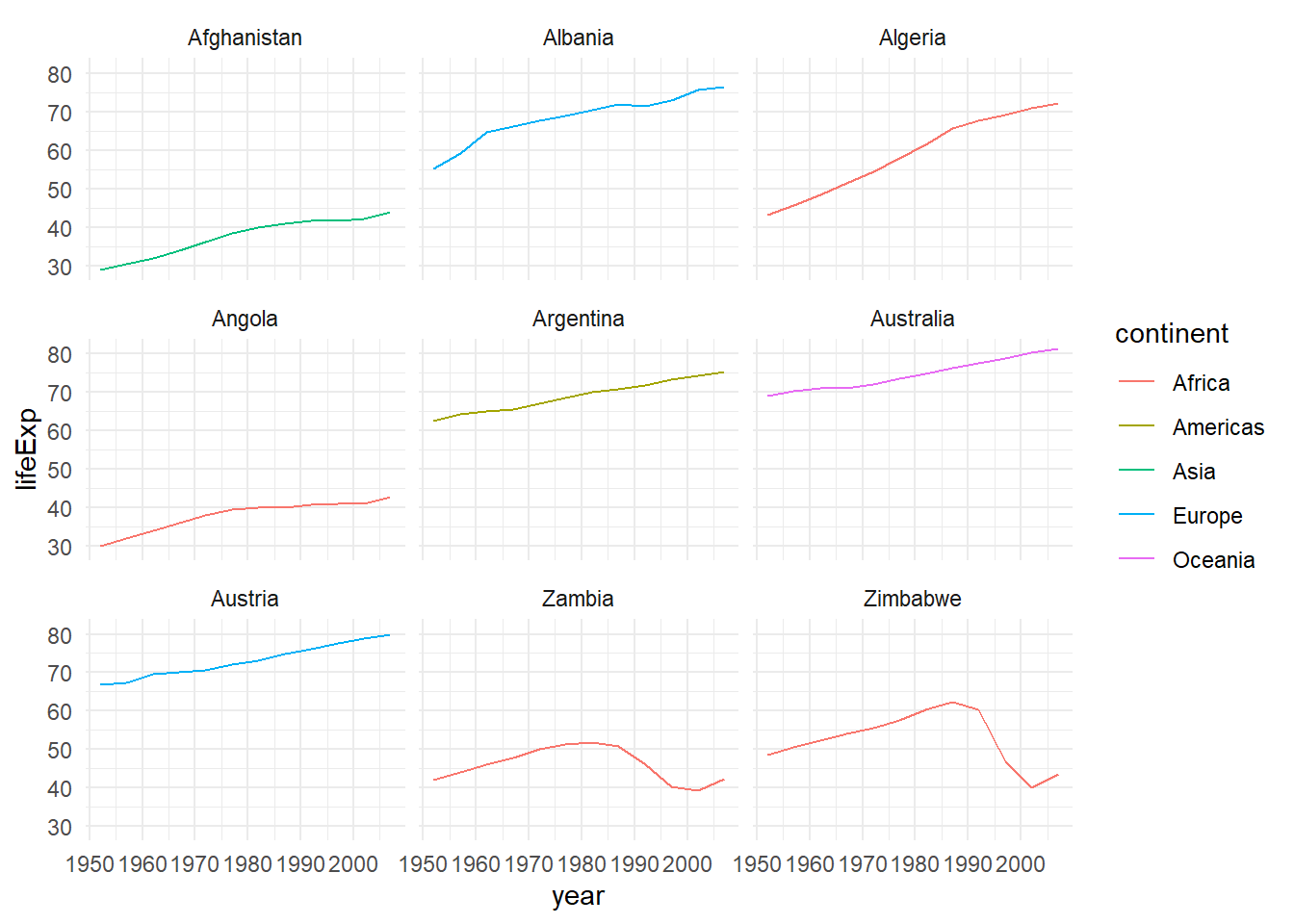
Combining mutate and ggplot2
Create new columns and plot in one pipeline:
%>% mutate (startsWith = substr (country, 1 , 1 )) %>% filter (startsWith %in% c ("A" , "Z" )) %>% ggplot (aes (x = year, y = lifeExp, colour = continent)) + geom_line () + facet_wrap (vars (country)) + theme_minimal ()
Advanced Challenge
Calculate the average life expectancy in 2002 of 2 randomly selected countries for each continent.
Then arrange the continent names in reverse order.
Hint: Use the dplyr functions arrange() and sample_n().
Advanced Challenge Solution
set.seed (42 ) # For reproducibility <- gapminder %>% filter (year == 2002 ) %>% group_by (continent) %>% sample_n (2 ) %>% summarize (mean_lifeExp = mean (lifeExp)) %>% arrange (desc (mean_lifeExp))
# A tibble: 5 × 2
  continent mean_lifeExp
  <chr>            <dbl>
1 Oceania           79.7
2 Asia              75.9
3 Europe            75.9
4 Americas          74.3
5 Africa            59.8
Key dplyr Verbs Summary
select()Choose columns
filter()Choose rows
group_by()Group data
summarize()Calculate summaries
mutate()Create new columns
arrange()Sort rows
count()Count observations
rename()Rename columns
Key Points
Use the dplyr package to manipulate data frames
Use select() to choose variables from a data frame
Use filter() to choose data based on values
Use group_by() and summarize() to work with subsets of data
Use mutate() to create new variables
Use pipes (%>%) to chain operations together
Important Reminders
Order of operations matters when combining select() and filter()
group_by() changes the data frame structuren() returns the count of observations in the current groupPipes make code more readable and reduce intermediate variables
Combine dplyr with ggplot2 for powerful data visualization workflows